Quick start

This walkthrough uses small illustrative data so you can learn what the plots mean before processing a real dataset. The example Newick is supplied for practice; it is not a tree inferred from the numbered arrays.

1. Plot three arrays

Download example-arrays.txt, or paste:

strain_A    1,2,3,6,7,9
strain_B    1,2,4,6,8,9
strain_C    10,2,4,6,8

1. Open SpacerMap from Analysis.
2. Paste the text or upload the file, using only one input method.
3. Keep Right alignment and explicitly select No clustering (the page initially selects Shared spacer).
4. Select Commit.

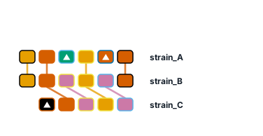
You should see three rows, 9 distinct spacer labels and 6 shared labels. There are 17 spacer occurrences in total. IDs 3 and 7 occur only in strain A; ID 10 occurs only in strain C. Those array-specific types are triangles. Shared types connect across neighboring rows where applicable.

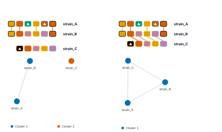
Try Ancestral spacer and wait for the automatic preview update: A and B share the rightmost ID 9, while C ends in 8 and forms its own group. Then try Shared spacer: all three arrays connect because every pair shares at least two distinct IDs. Show cluster network displays those links. This illustrates that different grouping rules answer different questions. Preview-only layout changes do not overwrite the saved job; download the current SVG or commit again to save a new result.

Choose SVG and Download SVG in the array-map export controls. Download numbered file is unnecessary for already numbered input; retain the example TXT.

Next, open Spacer occurrence → Show occurrence chart. IDs 2 and 6 should each have a bar height of 3; IDs 1, 9, 4 and 8 should each have height 2; IDs 3, 7 and 10 should each have height 1. In the matrix below the bars, filled circles mean present and hollow circles mean absent. Each array counts once per ID, even if that ID is repeated within it.

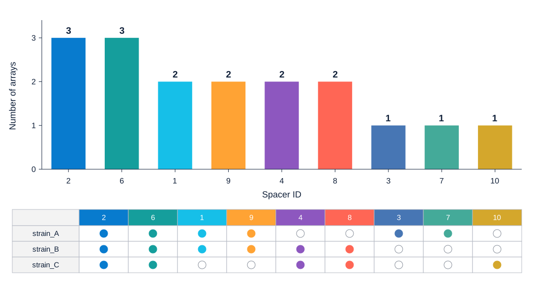
Select Download statistics CSV and compare it with the expected counts. Use this panel's own Format control to export the combined bar chart/matrix as SVG, PDF or another supported format. These statistics count arrays, not strains or total spacer copies. See the SpacerMap guide for the 50-ID chart limit and full interpretation.

2. Combine the arrays with a tree

Download example-tree.nwk, or copy:

((strain_A:0.12,strain_B:0.08)95:0.05,strain_C:0.18);

1. Open ArrayPhyloViz.
2. Add the tree under Phylogenetic tree.
3. Add the same arrays under CRISPR arrays, using the TXT or your exported SpacerMap SVG.
4. Select Exact names, then Commit.
5. Open Review and edit mapping: all three arrays should map to three leaves, with none unassigned.
6. Adjust row spacing and label space. Turn on Use branch lengths to compare proportional lengths with the default topology layout.
7. Keep the private link created by Commit. After edits, use Save changes again or Save project for a local JSON, then export SVG, PNG or PDF.

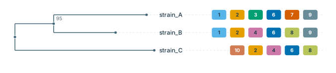
The tree groups A and B together. The array track helps inspect which types they share with each other and C. The internal label 95 came from the example tree; the editor did not calculate support. Reopen the saved JSON with Open saved project to continue editing.

3. Try data preparation and inference

For a detector-free trial, open CRISPRPrep → Load example → Import JSON results, keep the defaults and select Run. Examine retained/filtered arrays and the processed-row preview, then download Processed CSV and the report. To compare a different filter, load Import JSON results from Load example again (this resets options), change that filter and select Run for a new job. Keep a record of the settings for each result.

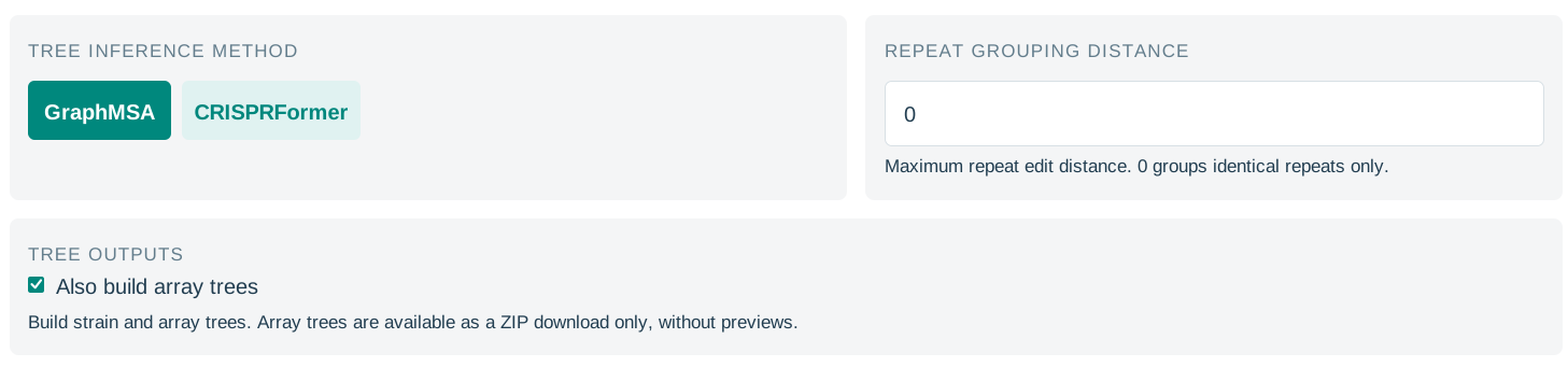
To try tree inference, open CRISPRPhylo → Load example, keep GraphMSA, then select Commit. This requires the site's inference service and can take time. Inspect the Newick source and download .nwk. Leave Repeat grouping distance at 0 for this first trial. Enable Also build array trees before submission if you also want the group-level ZIP. Do not substitute the other tools' built-in example buttons for this page's pasted three-array/Newick walkthrough: SpacerMap and ArrayPhyloViz load different examples. For your own cross-tool run, transfer or upload the same processed CSV and verify sample names.

4. Try sequence retrieval or target searching

SeqFetcher → Load example → Commit retrieves example nucleotide records from NCBI. Check metadata, keep the private results link, and download FASTA/ZIP for your records. For a whole-genome assembly, enter its GCA_/GCF_ accession with Nucleotide selected; one retrieved row may contain multiple FASTA contigs. These examples demonstrate retrieval, not bacterial CRISPR detection.

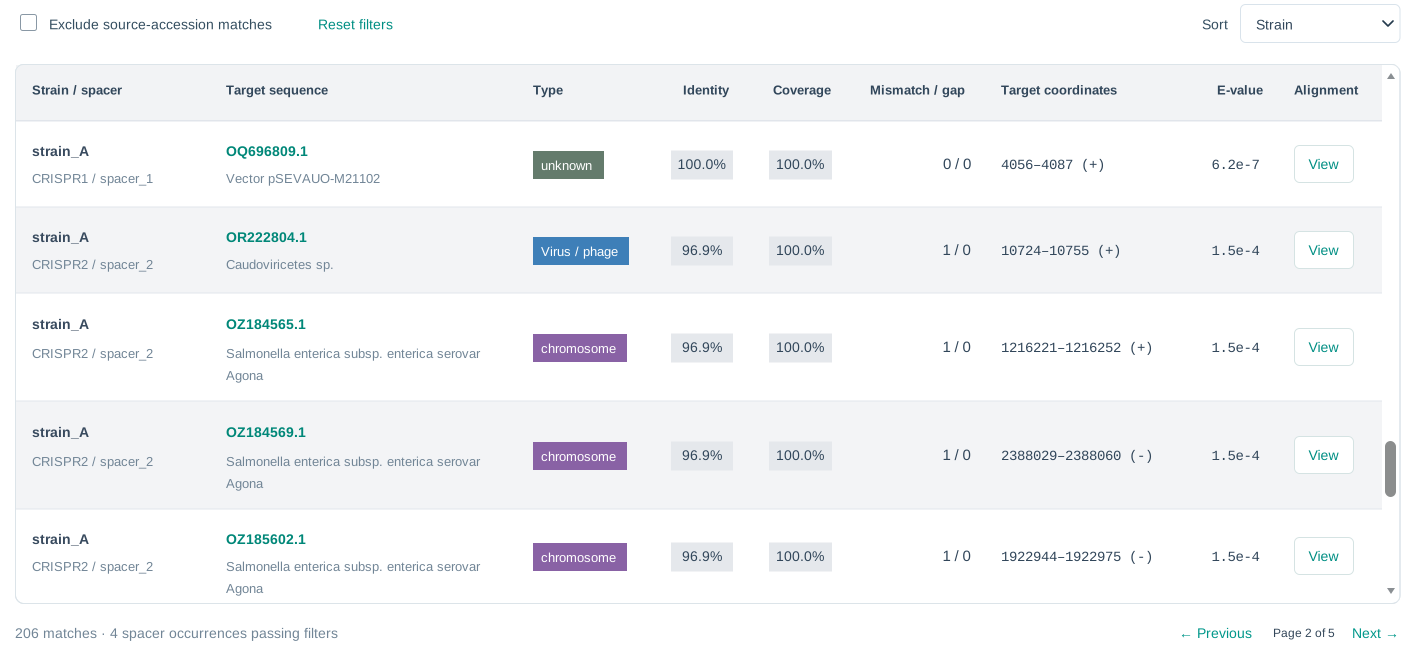
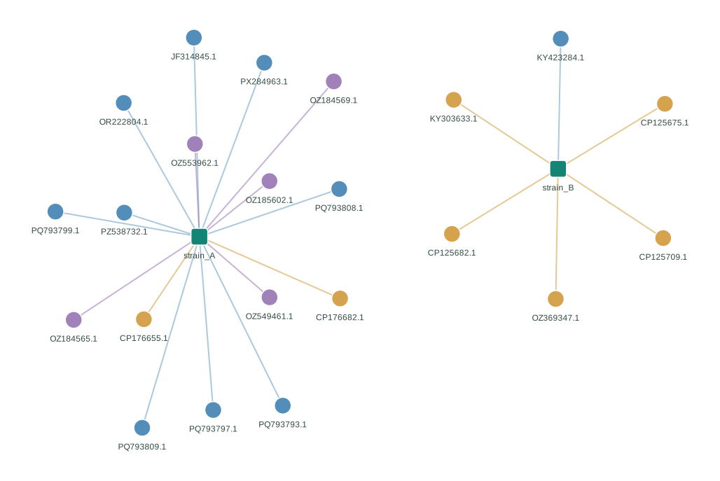
For SpacerTarget, use Load example or example-spacers.fasta, review the settings, then select Search. This submits a real NCBI search. Save Copy results link. Results depend on the database and search time, so no fixed hit count is expected. Follow the SpacerTarget guide to interpret Strict/Exact filters and network edges.

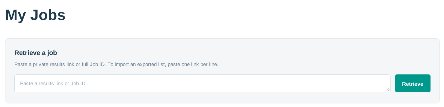
After a job is accepted, test recovery by copying its link into My Jobs → Retrieve a job. Open the result and confirm it is the expected dataset. Downloads and original inputs are still needed for long-term storage because server results expire after seven days.

Continue with the real-data workflow once input names and result types are familiar.